Implementing Smoothlife: A Tutorial
Recommended listening: Wincing The Night Away by The Shins
Introduction
Several years ago I learned about smoothlife, a continuous version of Conway's Game of Life. The original "Game of Life" was one of the things that motivated me to learn programming, and this other, more advanced version was similarly inspiring. I wanted to implement it eventually, once I learned the math required to understand how it works. I finally got around to doing so last semester, and it was an excellent distraction from final exams.
When researching how to implement smoothlife, I was dissatisfied with the state of literature on the topic (where "literature" means blog posts and GitHub READMEs). While there was evidently enough information that I was able to piece together a working program, I couldn't find a tutorial that said how to implement all of it, from start to finish. The original paper was clearly enough for some math wizards to figure out how to program smoothlife, but many people don't have such a deep mathematical background. While I hope this tutorial will be sufficient for ordinary programmers like myself, I know it won't be perfect.
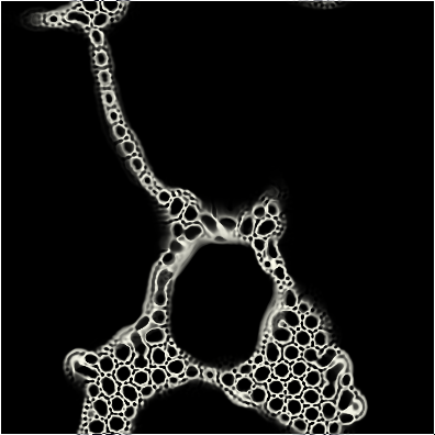
Before we go any further, it would help to clarify what smoothlife actually looks like. Here's a gif of the simulation in action, with the configuration
  BIRTH_1 = 0.269, BIRTH_2 = 0.34, DEATH_1 = 0.523,
  DEATH_2 = 0.746, RADIUS = 4.0, OUTER_RADIUS = (3.0 * RADIUS),
  BOUNDARY = 1.0, SPEED = 0.2
My code for smoothlife is hosted here. As mentioned in that repository, I consulted a few resources as I tried to wrap my head around things. This Python programis a good reference for how to implement the math, although it's a bit simplified; I also read the popular 0fps article for a deeper explanation of how the simulation works. The discretization method in that article is a little more complicated than what I used. I'd recommend reading that article first, as well as Rafler's original paper, at least to get the general idea of what smoothlife is.
First Steps: SDL2
To start, let's set up code to display a window. We'll be doing this in C, but you can probably get away with implementing smoothlife in any mainstream language, except maybe SQL. If you want to stick close to what I do in this tutorial, you'll need to have SDL2 installed for graphics, as well as FFTW for numerical computation.
Now for the actual code. Put this in a file called smooth.c and compile it by running gcc -Wall -g -O2 -lSDL2 smooth.c -o smooth:
#include <SDL2/SDL.h>
#include <stdio.h>
#include <stdlib.h>

#define SIZE 400
#define SCALE 1
#define SCREEN_SIZE (SIZE * SCALE)


int
main()
{
        SDL_Window *win = NULL;
        SDL_Renderer *ren;
        SDL_Event event;

        if (SDL_Init(SDL_INIT_VIDEO) < 0) {
                printf("SDL had an error: %s\n", SDL_GetError());
                return 0;
        }

        SDL_CreateWindowAndRenderer(SCREEN_SIZE, SCREEN_SIZE, 0, &win, &ren);

        while (1) {
                /* exit main loop when window is closed */
                if (SDL_PollEvent(&event) && event.type == SDL_QUIT)
                        break;

                SDL_RenderPresent(ren);
        }


        SDL_DestroyRenderer(ren);
        SDL_DestroyWindow(win);
        SDL_Quit();
        return 0;
}
This opens a blank window. What's important are the constants SIZE, SCALE, and SCREEN_SIZE. These three constants will define, respectively, the size of the "world," the size of a cell, and the size of the window.
A Donut-Shaped Field
Next, we need to figure out how to implement the formulas from Rafler's paper. You read it, right? In short, the simulation lives in a "world," which is a +discrete grid+ continuous field of cells, shaped like the surface of a torus. The torus part is mostly just a funny detail, because we're not mathematicians, and it won't do us any harm to pretend the field is a square. Also, the field isn't really continuous, because we're working on a computer, and can only simulate continuous things up to a certain (possibly high) resolution. Each cell has a floating-point value between 0 and 1, representing how dead or alive the cell is. Armed with that knowledge, we can initialize a two-dimensional array of doubles, which will be our (definitely continuous) field of cells:
#include <SDL2/SDL.h>
#include <stdio.h>
#include <stdlib.h>

#define SIZE 400
#define SCALE 1
#define SCREEN_SIZE (SIZE * SCALE)


int
main()
{
        SDL_Window *win = NULL;
        SDL_Renderer *ren;
        SDL_Event event;

        if (SDL_Init(SDL_INIT_VIDEO) < 0) {
                printf("SDL had an error: %s\n", SDL_GetError());
                return 0;
        }

        SDL_CreateWindowAndRenderer(SCREEN_SIZE, SCREEN_SIZE, 0, &win, &ren);


        double field[SIZE][SIZE];


        while (1) {
                /* exit main loop when window is closed */
                if (SDL_PollEvent(&event) && event.type == SDL_QUIT)
                        break;

                SDL_RenderPresent(ren);
        }


        SDL_DestroyRenderer(ren);
        SDL_DestroyWindow(win);
        SDL_Quit();
        return 0;
}
Convoluted Kernels, Part I
Every time-step of the simulation, the cells are updated, and are given a new state between 0 and 1. How is that new state determined? In the original Game of Life, a cell's new state is determined by its current state and the states of eight adjacent cells. In smoothlife, we replace this with the state of the cell's "inner neighborhood" (a smooth disc) and the state of its "outer neighborhood" (an annulus, which is like a circular ring).
How do we translate these shapes into code? Each neighborhood can be thought of as an array with SIZE * SIZE entries, the same size as the cell field, with values between 0 and 1. Entries within the neighborhood have a value of 1 (or close to 1), and entries outside the neighborhood have a value of 0. When calculating a cell's neighborhood, the neighborhood array is centered over the position of that cell, and then all cells in the field are multiplied by their corresponding neighborhood value, added up, and averaged.
In technical terms, the neighborhood array is called a kernel, and the process of taking its sum around every cell is called kernel convolution. It might seem like this would be a slow and inefficient process — you have to sum a grid of n coefficients for every cell in a size-n field — but there's a very fast way of doing it. Kernel convolution is performed all the time in "the real world," for things like image processing, and is a well-researched topic; and, luckily for us, mathematicians have discovered something called the convolution theorem which allows us to convolve things with extreme efficiency. This theorem states that you can take the Fourier transform of a kernel, multiply it element-wise by the Fourier transform of a grid, and inverse Fourier transform to get the result. In other words, K∗G = F^-1(F(K) ⋅ F(G)), where K is the kernel, G is the grid (aka field), F is the Fourier transform, ∗ is the convolution operator, and ⋅ is the element-wise multiplication operator. With all that math, you may wonder why I didn't choose to implement smoothlife in Python or M*TLAB. So do I.
That was a lot of talking, though. What does the code look like? First, here's a function for creating a disc-shaped kernel (compile with gcc -Wall -g -O2 -lSDL2 -lm smooth.c -o smooth):
#include <math.h>
#define BOUNDARY 1.0

double
disc_kernel(int radius, double kernel[SIZE][SIZE])
{
        double sum = 0.0f;

        for (int i = 0; i < SIZE; i++) {
                for (int j = 0; j < SIZE; j++) {
                        double di = i - (SIZE/2), dj = j - (SIZE/2);
                        double d = hypot(di, dj);
                        double n;

                        /* do anti-aliasing near the boundaries */
                        if      (d > radius + (BOUNDARY/2)) n = 0.0f;
                        else if (d < radius - (BOUNDARY/2)) n = 1.0f;
                        else n = (radius + (BOUNDARY/2) - d) / BOUNDARY;

                        sum += n;

                        /* "roll" indices to extreme edges */
                        int x = i;
                        int y = j;
                        x = (i + (COLS/2)) % COLS;
                        y = (j + (ROWS/2)) % ROWS;

                        kernel[x][y] = n;
                }
        }

        return sum;
}
A few things to note: This function returns the sum of coefficients inside the disc, which is useful for taking the average neighborhood state. We also "roll" the disc so that it's centered around the origin, so that the convolution works out as it's supposed to. Also, the disc is anti-aliased near the edges, so the transition from 1 to 0 looks "smooth". Anti-aliasing isn't crucial, but it looks nice.
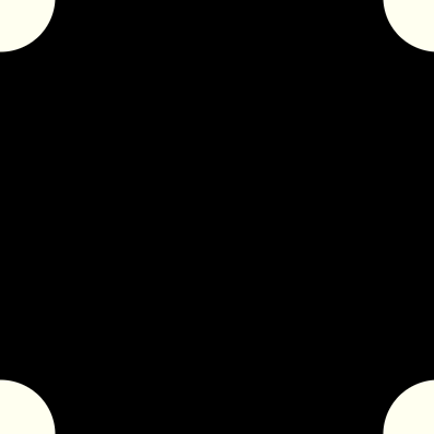
We now have code for initializing a disc-shaped kernel, but we still need to set up the annulus-shaped kernel. Thankfully, we can just subtract a small disc kernel from a larger disc kernel to obtain an annulus, reusing the disc_kernel function. Below is the code for initializing both kernels, which can go near the top of main:
#define RADIUS 4.0
#define OUTER_RADIUS (3.0 * RADIUS)

double ker_inner[SIZE][SIZE];
double ker_outer[SIZE][SIZE];
double inner_area = disc_kernel(RADIUS, ker_inner);
double outer_area = disc_kernel(OUTER_RADIUS, ker_outer);

/* punch an inner-kernel-shaped hole in the outer kernel */
outer_area -= inner_area;
for (int i = 0; i < SIZE; i++) {
        for (int j = 0; j < SIZE; j++) {
                ker_outer[i][j] -= ker_inner[i][j];
        }
}
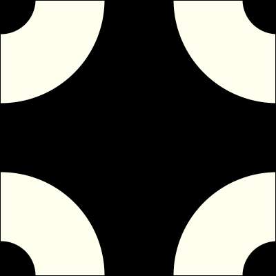
Here are some pictures of the inner and outer kernel, centered around the origin:
The Fastest FFT in the West
Now that we know how to generate the kernels, we need code for performing the fast Fourier transform (and its inverse). Luckily, there's a C library for computing FFTs, as alluded to earlier; unfortunately, it's a bit of work to use. First, the function for the forward FFT (compile with gcc -Wall -g -O2 -lSDL2 -lm -lfftw3 smooth.c -o smooth):
fftw_complex
*forward_fft(int w, int h, double data[w][h], unsigned mode)
{
        double *in;
        double complex *out;
        fftw_plan p;

        in  = fftw_malloc(sizeof (*in) * w * h);
        out = fftw_malloc(sizeof (*out) * w * (1 + h/2));
        p = fftw_plan_dft_r2c_2d(w, h, in, out, mode);

        for (int n = 0; n < w * h; n++) {
                int i = n % w, j = n / w;
                in[n] = data[i][j];
        }


        fftw_execute(p);

        fftw_destroy_plan(p);
        fftw_free(in);


        return out;
}
It's not strictly necessary to understand what goes on here, but I'll point out some of the stranger parts anyway. The function transforms a 2-dimensional grid of real numbers (field, kernel, etc) of size w*h. Funnily enough, the output is a list of complex numbers of size w*(1 + h/2), which you can see in the call to fftw_malloc. We use the function fftw_plan_dft_r2c_2d to build a "plan" for transforming 2-dimensional real input data into an array of complex numbers. The plan also takes a mode parameter, which should either be FFTW_MEASURE or FFTW_ESTIMATE. The former is good if you want to spend some extra time optimizing the FFT, while the latter is better for frequently performed FFTs. Don't worry if the difference isn't clear, because it will become apparent soon. Before executing the FFT, we copy data into in, flattening the 2-dimensional array indices into a one-dimensional index. Then we execute the FFT and perform some cleanup; we'll have to free the output data at some later point.
Here's the inverse FFT code, just to get it out of the way. We won't use it until a little bit later on:
double
*backward_fft(int w, int h, double complex *in)
{
        double *out;
        fftw_plan p;

        out = fftw_malloc(sizeof (*out) * w * h);
        p = fftw_plan_dft_c2r_2d(w, h, in, out, FFTW_ESTIMATE);

        fftw_execute(p);

        fftw_destroy_plan(p);
        fftw_free(in);

        /* results need to be scaled down by array size */
        int size = w * h;
        for (int i = 0; i < size; i++) {
                out[i] /= size;
        }

        return out;
}
The only strange thing about this function, as long as you understand forward_fft, is that the result needs to be scaled down by dividing by its size. This is just a peculiarity of the FFT algorithm that FFTW uses.
Now we need to perform the forward FFT on our kernels. The kernels never change, so we only need to FFT them once, after they're initialized in main:
double complex *fft_inner = forward_fft(SIZE, SIZE, ker_inner, FFTW_MEASURE);
double complex *fft_outer = forward_fft(SIZE, SIZE, ker_outer, FFTW_MEASURE);

/* ... */
/* end of main */
fftw_free(fft_inner);
fftw_free(fft_outer);
Great Ssssnakes!
Next, we need to handle state transitions. Earlier I mentioned that a cell's "next" state is determined by its "current" state, and the average state of its neighbors. Unlike the discrete game of life, where cells can exist in two states (alive and dead), the cells in smoothlife exist between life and death, represented by a value between 0 and 1. The discrete update rule can be thought of as a simple step function, and we can smooth it out by using a continuous function with a similar shape to the discrete step. To do this, we can just combine a bunch of sigmoid functions together. A sigmoid function is basically an s-shaped curve with upper and lower asymptotes, and it's helpful for creating smooth transitions between two values. If you want to learn more about how it works, the 0fps article is an excellent resource.
To help visualize the difference between the discrete update function and its continuous analog, here are two (very rough) graphs of the respective functions. The update function operates on a single cell, and take that cell's state and neighborhood density as inputs. The vertical axis on these plots represents the cell's state, and the horizontal axis is the neighborhood density; the color of the pixel at each point represents the value of the update function for the inputs corresponding to the pixel's location, with white denoting "alive." These graphs depict the output of do_rule, defined a few paragraphs later.

#define ALPHA_N 0.028
#define ALPHA_M 0.147

double
logistic(double x, double a, double alpha)
{
        return 1.0 / (1 + exp((-4/alpha) * (x - a)));
}


double
threshold(double x, double a, double b)
{
        return logistic(x, a, ALPHA_N) * (1 - logistic(x, b, ALPHA_N));
}

double
interp(double x, double y, double m)
{
        return (x * (1 - logistic(m, 0.5, ALPHA_M))) +
                (y * logistic(m, 0.5, ALPHA_M));
}
ALPHA_M and ALPHA_N are parameters that control the "steepness" of certain transitions, and are actually quite important to get right. I'm using the values from the original paper here, as you'll find that changing these constants too much will result in muddled behavior. It's also important to use logistic interpolation in interp, because linear interpolation will result in undesirable behavior — in most cases, stable patterns will just expand to cover the whole field, which isn't very dynamic.
Then we have a function for applying the "rule" to each cell, updating it based on its neighborhood and current state. The BIRTH and DEATH constants are very important, because the behavior of the simulation depends on them. These are fun parameters to play around with, and a great range of behavior can be observed for different configurations.
#define BIRTH_1 0.257
#define BIRTH_2 0.336
#define DEATH_1 0.380
#define DEATH_2 0.465

double
do_rule(double state, double neighbs)
{
        return threshold(neighbs, interp(BIRTH_1, DEATH_1, state),
                         interp(BIRTH_2, DEATH_2, state));
}
Convoluted Kernels, Part II
Next, we need to tie all this math together, and create our function for updating the field. An update basically consists of convolving the field with both kernels, and then applying the update function to each value in the result. Remember that we're using the convolution theorem, though, so we need to perform more Fourier transforms. To do this, we'll make a helper function:
double
*fft_convolve(double complex *ker, double complex *field)
{
        /* multiply corresponding elements of "kernel" and field */
        int n = SIZE * (1 + SIZE/2);
        double complex *products = fftw_malloc(sizeof (*products) * n);

        for (int i = 0; i < n; i++) {
                products[i] = ker[i] * field[i];
        }

        /* perform inverse fft on the products */
        double *result = backward_fft(SIZE, SIZE, products);

        return result;
}
This function takes a kernel and a field, both results of a forward Fourier transform. The two arrays are multiplied together element-wise, and then the inverse FFT is applied. In terms of the convolution theorem, ker is F(K), field is F(G), and fft_convolve computes F^-1(F(K) ⋅ F(G)).
Now it's time to write the most complicated function. do_step updates the field of cells in one (discrete) time-step. It takes the two kernels, already FFT'd, as well as the area of each kernel. Then it takes the current field of cells, as well as an array that holds the next field of cells. The current field is FFT'd and convolved with both kernels, and then the update rule is applied to each cell.
void
do_step(double inner_area, double outer_area,
        double complex *fft_inner, double complex *fft_outer,
        double cell_field[SIZE][SIZE], double next_field[SIZE][SIZE])
{
        double complex *fft_field =
                forward_fft(SIZE, SIZE, cell_field, FFTW_ESTIMATE);
        double *states = fft_convolve(fft_field, fft_inner);
        double *neighbs = fft_convolve(fft_field, fft_outer);

        for (int n = 0; n < SIZE * SIZE; n++) {
                /* normalize state and neighb values */
                double st = states[n]  / inner_area;
                double nb = neighbs[n] / outer_area;

                double s = do_rule(st, nb);
                int i = n % SIZE;
                int j = n / SIZE;

                next_field[i][j] = s;
        }

        fftw_free(fft_field);
        fftw_free(states);
        fftw_free(neighbs);
}
The Easy Part
We'll also need some utility functions for drawing and initializing the field of cells. First, here's a function that draws "splotches" of live cells onto the field:
void
splotch(int x, int y, int size, double cells[SIZE][SIZE])
{
        for (int i = 0; i < size; i++)
                for (int j = 0; j < size; j++)
                        cells[(x+i)%SIZE][(y+j)%SIZE] = 1.0f;
}
The rendering function is very simple; we just render each cell as a little square, and color it based on its life value. I also decided to color cells red if their life value is too low, and blue if their value is too high, in order to detect errors. It's useful for debugging, but in this version of smoothlife, cells simply don't go out of bounds :).
void
render_cell(SDL_Renderer *ren, double cell, int x, int y)
{
        SDL_Rect rect = (SDL_Rect){.x=x*SCALE, .y=y*SCALE,
                                   .w=SCALE, .h=SCALE};

        int c = 255 * cell;
        if (cell < 0) SDL_SetRenderDrawColor(ren, 255, 0, 0, 255);
        else if (cell > 1) SDL_SetRenderDrawColor(ren, 0, 0, 255, 255);
        else SDL_SetRenderDrawColor(ren, c, c, 240 * cell, 255);


        SDL_RenderFillRect(ren, &rect);
}
Finale
Let's add the finishing touches to main:
#include <time.h>
#define SPEED 0.2

/* init cells */
for (int x = 0; x < SIZE; x++)
        for (int y = 0; y < SIZE; y++)
                field[x][y] = 0.0f;

srand(time(NULL));
for (int i = 0; i < SIZE; i++) {
        for (int j = 0; j < SIZE; j++) {
                if ((rand() % 1000) <= 10)
                        splotch(i, j, 5, field);
        }
}


while (1) {
        /* exit main loop when window is closed */
        if (SDL_PollEvent(&event) && event.type == SDL_QUIT)
                break;

        /* draw and update all of the cells */
        double new_field[SIZE][SIZE];
        do_step(inner_area, outer_area, fft_inner, fft_outer, field, new_field);

        for (int x = 0; x < SIZE; x++) {
                for (int y = 0; y < SIZE; y++) {
                        double cell = field[x][y];
                        double   dc = new_field[x][y];

                        render_cell(ren, cell, x, y);
                        new_field[x][y] = cell + ((dc - cell) * SPEED);
                }
        }

        SDL_RenderPresent(ren);

        memcpy(field, new_field, sizeof(field));
}
We first initialize all cells in the field to state 0 (dead); then, we randomly add "splotches" of live cells. The time() function, from time.h, is used to seed the random number generator.
Every iteration of the the main loop, we perform a discrete time-step, and then loop through the cells to render and update them. An important detail here is that the cells in new_field are adjusted so that they approach the new state at a rate of SPEED, which gives the illusion of a "smooth" time-step. This is similar to (perhaps the same as) the Euler method, a technique which is used, among other things, for smooth time-steps in physics engines.
After that loop, the renderer is updated, and the new field is copied into the old one. And that's it! The simulation should look something like this when you run it: